Nils Malmberg - Projets

mdisd : une librairie C++/Python pour l'interpolation multi-dimensionnelle de données.

Contexte

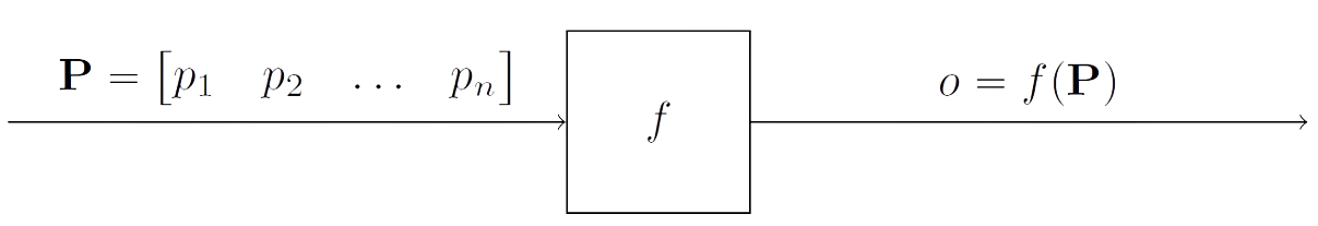
Considérons un système qui dépend directement de \(n\) paramètres et renvoie une quantité de sortie basée sur ces \(n\) paramètres. Par exemple, considérons une usine dont la quantité de sortie est la quantité de produits finis. Les paramètres d'entrée peuvent être, par exemple, la quantité de matériaux, l'état des machines, la fatigue des employés etc. L'usine est représenté par la fonction \(f\), le nombre de produits finis par \(o\) et les paramètres d'entrée par \(\textbf{P}\).

Il peut donc être difficile de créer un modèle qui prenne en compte tous ces paramètres afin d'estimer la quantité de produits finis pour l'état actuel de l'usine. C'est pourquoi la méthode proposée ici vise à interpoler la quantité de produits finis à partir d'une collecte de données effectuée au préalable et de l'état actuel de chacun des paramètres.

Approche

Pour ce faire, considérons que l'entreprise a pris soin de collecter les paramètres de l'usine et les quantités de produits finis correspondant à ces paramètres à plusieurs intervalles de temps différents (sur plusieurs jours, mois ou années). Considérons les \(m\) mesures de ces paramètres et des quantités de produits.

Une quantité connue de produit fini \(o_i\) peut donc être associée à un état correspondant de l'usine \(\textbf{P}_i\) for all \(i\) in \([\![1;m]\!]\). Ce qui donne en format matriciel:

\( \textbf{P} = \begin{pmatrix} \textbf{P}_1\\ \textbf{P}_2 \\ \vdots \\ \textbf{P}_m \end{pmatrix} = \begin{pmatrix} p_{1,1} & p_{1,2} & \cdots & p_{1,n} \\ p_{2,1} & p_{2,2} & \cdots & p_{2,n} \\ \vdots & \vdots & \vdots & \vdots\\ p_{m,1} & p_{m,2} & \cdots & p_{m,n} \end{pmatrix}\) \( \textbf{O} = \begin{pmatrix} o_1\\ o_2 \\ \vdots \\ o_m \end{pmatrix} = \begin{pmatrix} f(\textbf{P}_1)\\ f(\textbf{P}_2) \\ \vdots \\ f(\textbf{P}_m) \end{pmatrix} \)

L'objectif est maintenant d'estimer une nouvelle sortie \(o_{\text{new}} = f(\textbf{P}_{\text{new}})\) à partir d'une nouvelle entrée \(\textbf{P}_{\text{new}} = \begin{pmatrix} p_{\text{new,1}} & p_{\text{new,2}} &\dots & p_{\text{new,n}}\end{pmatrix}\).

Moindres Carrés Ordinaires/Ordinary Least Squares

La méthode des moindres carrés ordinaires (MCO ou OLS en anglais) est une méthode fondamentale de modélisation statistique utilisée pour estimer la relation entre une variable dépendante et une ou plusieurs variables indépendantes. Elle consiste essentiellement à minimiser la somme des carrés des différences entre les valeurs observées et prédites. Ainsi, les MCO visent à trouver la droite (dans la régression linéaire simple) ou le plan/hyperplan (dans la régression multivariée) qui s'ajuste le mieux aux points de données observés.

\[ \widehat{o}_\text{new} = \widehat{\alpha} + \sum\limits_{i=1}^n \widehat{\beta}_i \times p_{\text{new},i}\\ \]

L'idée principale derrière cette méthode est de trouver les coefficients \(\widehat{\alpha}, \widehat{\beta}_1, \cdots, \widehat{\beta}_n\) minimisant la somme suivante dans l'optique d'avoir la plus petite distance entre les points connus et leurs estimations par regression:

\[ \sum\limits_{i=1}^m \left[o_i - \underbrace{\left(\widehat{\alpha} + \sum\limits_{i=1}^n \widehat{\beta}_i \times p_{\text{new},i}\right)}_{\widehat{o}_\text{new}}\right]^2 \]

Introduisons les notations matricielles suivantes:

\( X = \begin{pmatrix} 1 & p_{1,1} &p_{1,2} & \cdots & p_{1,n} \\ 1 & p_{2,1} &p_{2,2} & \cdots & p_{2,n} \\ \vdots & \vdots & \vdots & \vdots & \vdots\\ 1 & p_{m,1} &p_{m,2} & \cdots & p_{m,n} \\ \end{pmatrix}\) \(\widehat{\beta} = \begin{pmatrix} \widehat{\alpha} \\ \widehat{\beta}_1 \\ \vdots \\ \widehat{\beta}_n \end{pmatrix}\) \(O = \begin{pmatrix} o_1\\ o_2 \\ \vdots \\ o_m \end{pmatrix} \)

Ainsi, les coefficients minimisant la somme sont:

\[ \widehat{\beta} = \left(X^T X\right)^{-1} X^T O \]

Fonction à Base Radiale/Radial Basis Function

Idée : chaque point défini par \(\textbf{P}_i\) and \(o_i\) "influence" sont voisinage dans chaque direction de manière identique selon la fonctionnelle \(\phi(r)\) où \(r\) est la distance radiale.

\[ o_\text{new} = \sum\limits_{i=1}^m \omega_i\cdot \phi(||\textbf{p}_\text{new} - \textbf{p}_i||) \]

Pour déterminer les poids \(w_i\), nous devons résoudre le système linéaire à \(m\) equations afin d'imposer que l'interpolation d'un point connu donne exactement la solution connue:

\[ \forall i\in [\![1;m]\!],~~~~ o_i = \sum\limits_{k=1}^m \omega_k\cdot \phi(||\textbf{p}_i - \textbf{p}_k||) \]

Le système peut être écrit sous la forme matricielle suivante:

\[\Phi \Omega = O\]

où, \(\Phi = \left[\phi(||\textbf{P}_j-\textbf{P}_i||)\right]_{(i,j)\in[\![1,m]\!]^2}\) (ligne i, colonne j)

et \(\Omega = \begin{pmatrix} \omega_1 & \omega_2 & \cdots & \omega_m\end{pmatrix}^T\) (T désigne la transposée)

Résultats

Ce projet a conduit au développement de la bibliothèque mdisd, qui peut être utilisée pour appliquer les MCO (moindres carrés ordinaires), la RBF (fonction de base radiale) et d'autres méthodes telles que la NRBF (RBF normalisée) et la RBFP (RBF augmentée par des polynômes). Ce projet contient d'autres outils tels que des outils de mise à l'échelle et des fonctions de base radiales. Il génère également un fichier bibliothèque pour Python. Vous trouverez un rapport détaillé sur le Github de la bibliothèque dans le dossier doc/, ainsi que le code source et divers cas tests.

Retour Lien vers le Github du projet

mdisd: a C++/Python library for multi-dimensional interpolation of scattered data.

Context

Let's consider a system that depends directly on \(n\) parameters and returns an output quantity based on these \(n\) parameters. For example, consider a factory whose output quantity is the final product, or more precisely the quantity of finished products. The input parameters of this factory are, for example, the flow of raw materials, the state of fatigue of the employees, the state of the machines, and so on. The plant is represented by the function \(f\), the number of finished products by \(o\), and the input parameters by the vector \(\textbf{P}\).

It can therefore be difficult to create a model that takes all these parameters into account in order to estimate the quantity of finished products for the current state of the plant. For this reason, the method proposed here aims to interpolate the quantity of finished products from a collection of data made beforehand and from the current state of each of the parameters.

Approach

To do this, let's consider that the company has taken care to collect the factory parameters and the quantities of finished products corresponding to these parameters at several different time intervals (over several days, months, or years). Consider \(m\) measurements of these parameters and product quantities.

A known quantity of finished product \(o_i\) can therefore be associated with the corresponding state of the plant \(\textbf{P}_i\) for all \(i\) in \([\![1;m]\!]\). In matrix format, this gives:

The aim now is to estimate a new output \(o_{\text{new}} = f(\textbf{P}_{\text{new}})\) from a new input \(\textbf{P}_{\text{new}} = \begin{pmatrix} p_{\text{new,1}} & p_{\text{new,2}} &\dots & p_{\text{new,n}}\end{pmatrix}\).

Ordinary Least Squares

Ordinary Least Squares (OLS) is a fundamental method in statistical modeling used to estimate the relationship between a dependent variable and one or more independent variables. Its essence lies in minimizing the sum of the squared of the differences between the observed and predicted values. Thus, OLS aims to find the line (in simple linear regression) or plane/hyperplane (in multivariate regression) that best fits the observed data points.

\[ \widehat{o}_\text{new} = \widehat{\alpha} + \sum\limits_{i=1}^n \widehat{\beta}_i \times p_{\text{new},i}\\ \]

The main idea behind the ordinary least squares method is to choose the coefficients \(\widehat{\alpha}, \widehat{\beta}_1, \cdots, \widehat{\beta}_n\) to minimize the following sum in order to have the smallest distance between the known points and the estimates of these same points by regression:

\[ \sum\limits_{i=1}^m \left[o_i - \underbrace{\left(\widehat{\alpha} + \sum\limits_{i=1}^n \widehat{\beta}_i \times p_{\text{new},i}\right)}_{\widehat{o}_\text{new}}\right]^2 \]

Let's introduce the following matrix notations:

Then, the coefficients that minimizes the sum are

\[ \widehat{\beta} = \left(X^T X\right)^{-1} X^T O \]

Radial Basis Function

Idea : each point defined by \(\textbf{P}\) and \(\textbf{O}\) "influences" its surroundings in the same way and in all directions according to the functionnal form \(\phi(r)\) where \(r\) is the radial distance.

\[ o_\text{new} = \sum\limits_{i=1}^m \omega_i\cdot \phi(||\textbf{p}_\text{new} - \textbf{p}_i||) \]

To determine the weights \(w_i\), we have to solve the \(m\) linear equations to impose that the interpolation is exact at all known data points:

\[ \forall i\in [\![1;m]\!],~~~~ o_i = \sum\limits_{k=1}^m \omega_k\cdot \phi(||\textbf{p}_i - \textbf{p}_k||) \]

This system can be written in the following matrix form:

\[\Phi \Omega = O\]

where, \(\Phi = \left[\phi(||\textbf{P}_j-\textbf{P}_i||)\right]_{(i,j)\in [\![1;m]\!]^2}\) (row: i, column: j)

and \(\Omega = \begin{pmatrix} \omega_1 & \omega_2 & \cdots & \omega_m\end{pmatrix}^T\) (transpose: T)

Results

This project led to the development of the mdisd library, which can be used to apply OLS (Ordinary Least Squares), RBF (Radial Basis Function) and other methods such as NRBF (Normalized RBF) and RBFP (RBF augmented with Polynomials). It contains other tools such as rescaling tools and radial basis functions. It also generates a library file for Python use. You'll find a detailed report on the library's Github in the doc/ folder, as well as source code and various test cases.

Back Link to the Github repository